View related contents

Related Help Topic
Calculating innings total runs after each over
Go back to activity
×
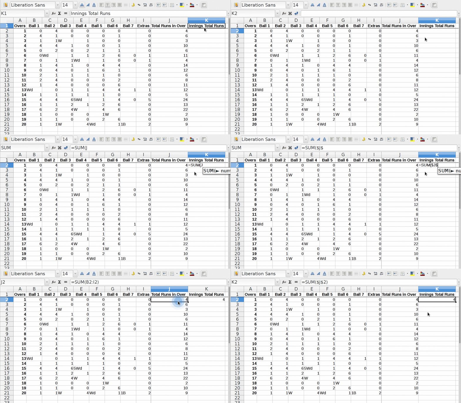
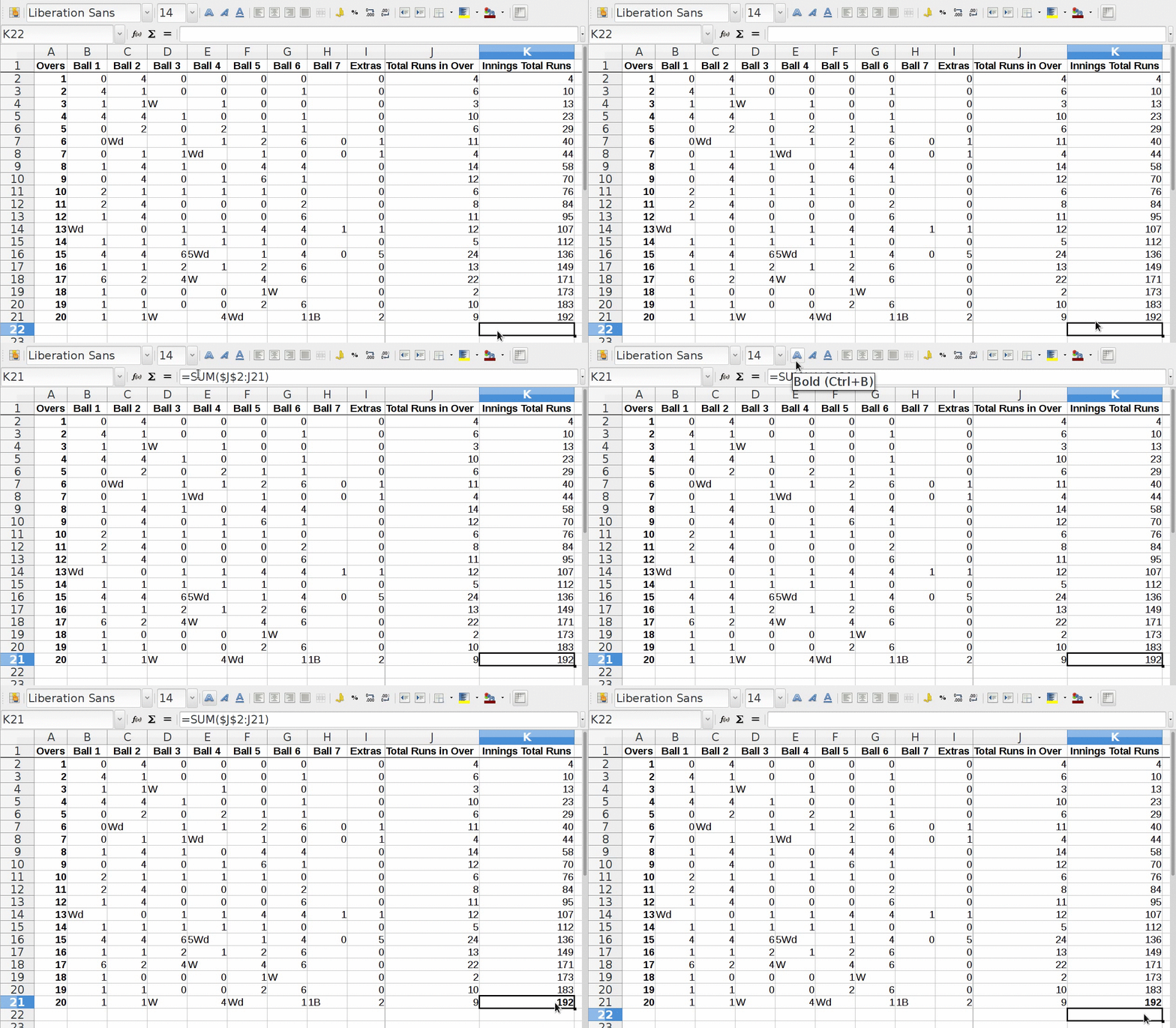
- To calculate innings total runs after each over, we have to add current over's runs into, innings total runs till it's previous over.
- For this, go to cell K2 in column “Innings Total Runs”
- Add “=SUM(” then "$" then "J" and then ":" and "$" then "2" and bracket ")" complete, as innings total runs after 1st over
- Then go to cell K3

Using "$" for cell range with fixed starting cell:
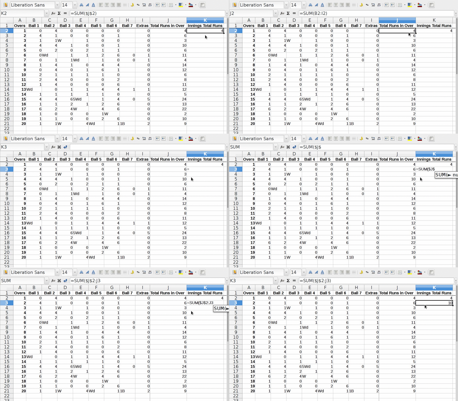
- Here from cell K3 till K21, we need to do the addition of cell range, starting from J2 till the cell of J column, intersecting in corresponding row.
- Example:
- Cell value of K3 = J2 + J3
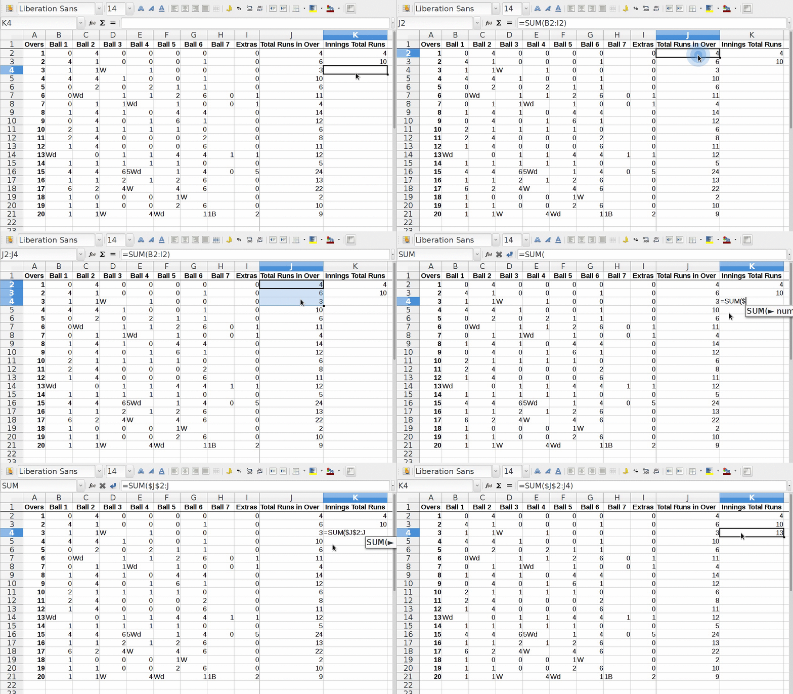
- Cell Value of K4 = J2 + J3 + J4
- ....
- Cell Value of Kn = J2 + J3 + J4 + ....... + Jn
- From this we conclude that, for each total, cell range is starting from cell J2.
- For keeping fix part in cell range we prefix $ to that fix part.
- Add formula in cell K3 as "SUM=", the in bracket "(" write as $, then append "J", then "$" and append "2", after this put colon ":" and "J3" and press enter. (Notice $ sign)
- Now you can use auto-completion to reflect innings total for remaining cells of column or apply once again same formula modified according to row number, to see how, go to next step.

- Add formula in cell K4 as "SUM=", the in bracket "(" write as $, then append "J", then "$" and append "2", after this put colon ":" and "J4" and press enter. (Notice $ sign)

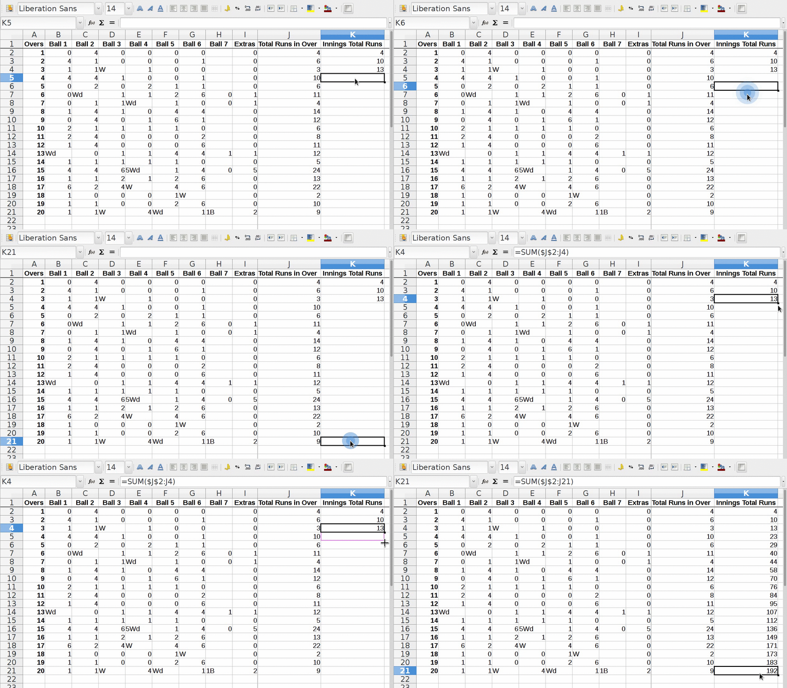
- Now use auto-completion to reflect innings total for remaining cells of column.

Making Innings final total as Bold:
- For making innings total runs bold go to last cell of column "Innings Total Runs" i.e. K21
- Press "Ctrl + B" key combination.

Related Help Topic
Making data entry into table
Go back to activity
×
Table in a spreadsheet means, combination of rows and columns.
Entering "over numbers" into "overs" column:
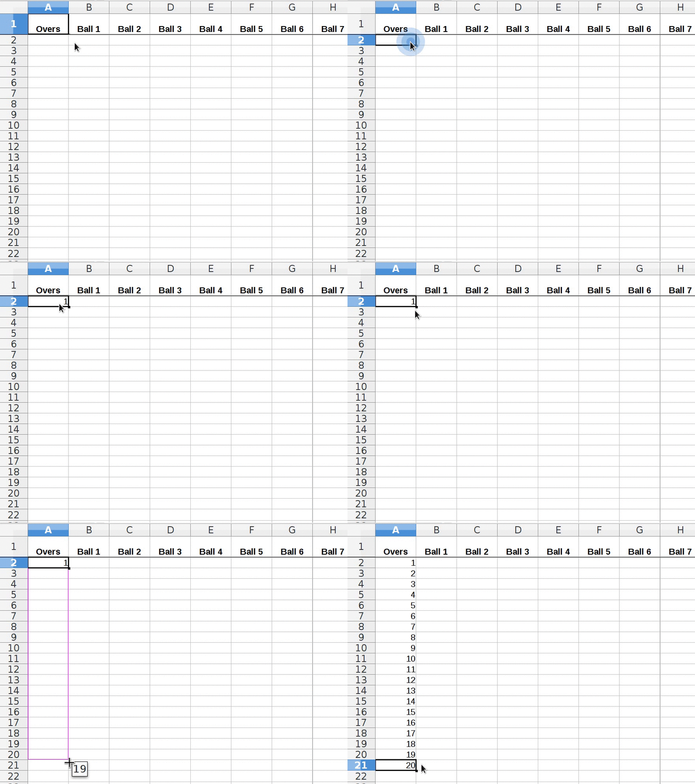
- Select the cell number "A2", enter number "1", which represents first over.
- After pressing "enter" button, again select the cell "A2", look for the tiny square, at the right bottom corner of the selected cell.
- Take your mouse pointer over that tiny square, and drag it, till row number "21".
- Since we need to insert data for 20 overs and first row is used for naming the columns, we need to use 21 rows.
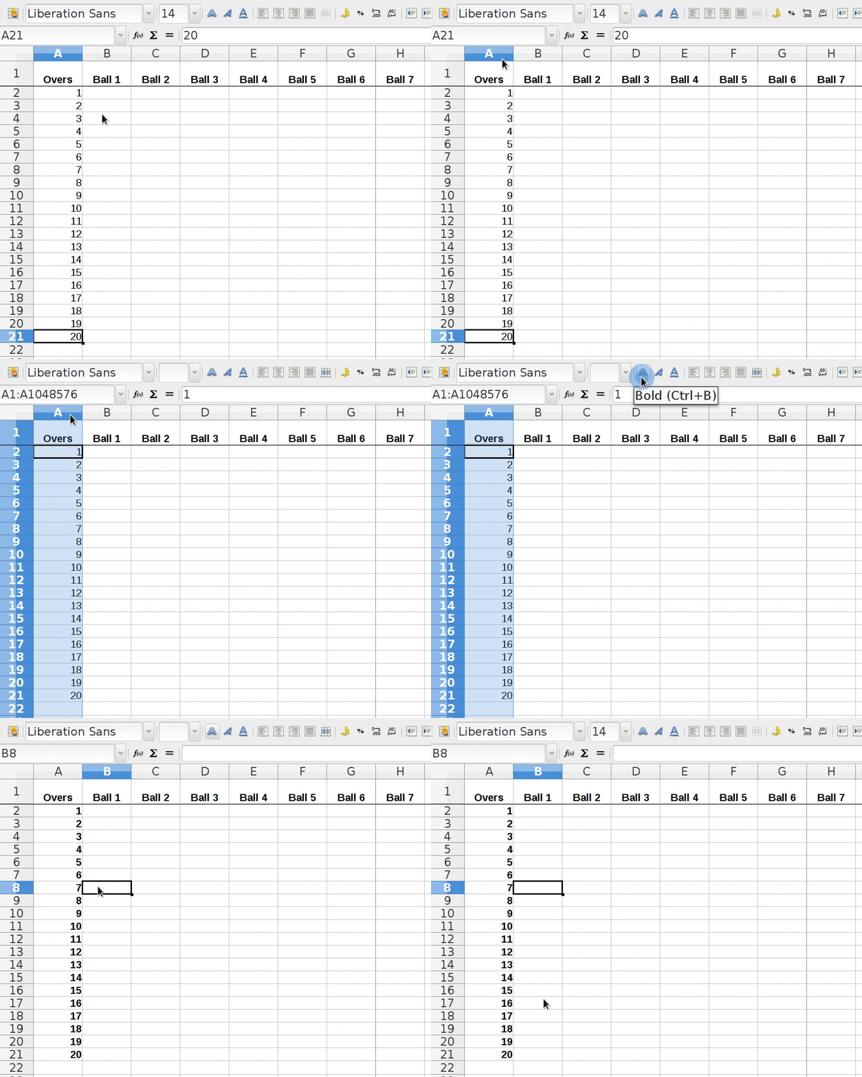
Make "over numbers" bold by selecting "Overs" column and press “Ctrl + B” key combination.
Related Help Topic
Adding runs per ball per over
Go back to activity
×
- Start adding runs for each ball in every over by selecting corresponding cell, starting from "B2" cell.
- Symbols for adding extra runs:
- If wicket is fallen, then enter "W" in the corresponding cell.
- If wide ball bowled, then enter "Wd" in the corresponding cell.
- If byes runs come, then apend "B" to the number of runs taken. (e.g. 2B : two byes runs taken)
- Likewise we will add the runs ball by ball for each over till 6th over.
- In the 6th over we come to know that 2nd ball of the over is wide ball.
- Because of this wide bowl, bowler has bowled one extra ball that is 7th ball of 6th over.
- But we made columns with the provision that, each over will have maximum 6 balls.
- So we need extra column, apart from existing ones, so lets go to next page to find out what to do.
Related Help Topic
Formatting cell for decimal points
Go back to activity
×
- After calculating run rate, for each over, we will see numbers with more than 2 decimal points, which is default setting
- We can change this to show numbers with max 2 decimal points
- For this select the column "Run rate" by clicking on its column header
- Then right click mouse and select Format Cells option
- A pop-up will get opened with Number as selected category
- Then go to Decimal Places in Options and replace 0 by 2 either by using upper arrow
- Press "OK" to apply the change
- Now you will see numbers with only two decimal points in Run Rate column.

Related Help Topic
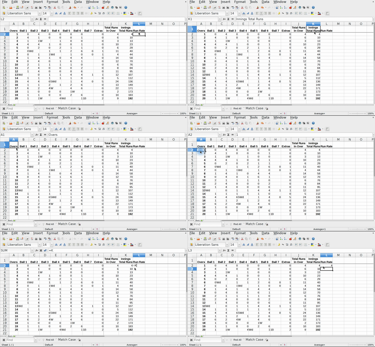
Calculate run rate
Go back to activity
×
- Run rate is nothing but average runs per over
- So we have to divide the innings total runs by number of completed overs.
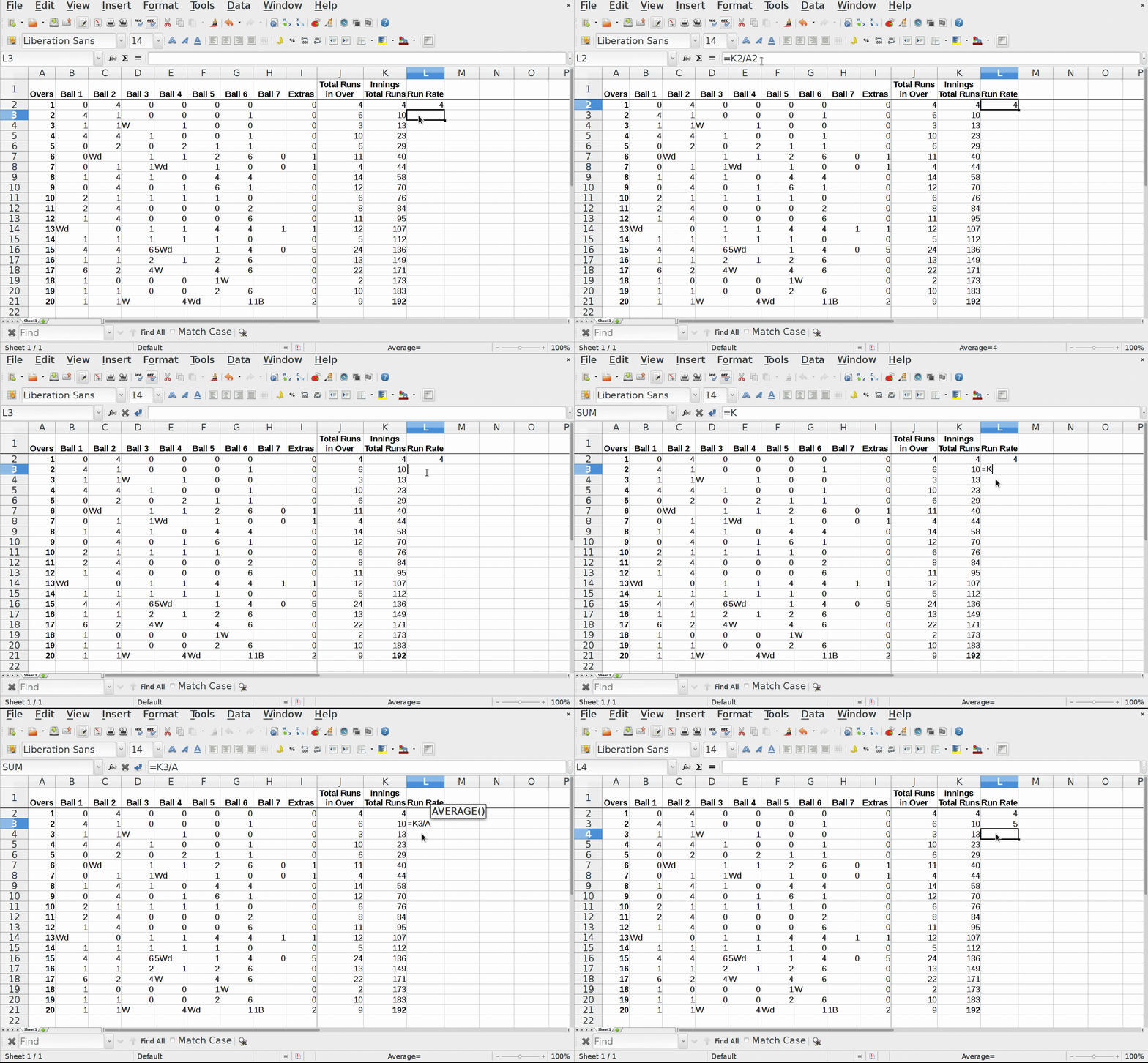
- Select cell L2 and enter the formula as =(K2/A2) and press enter
- Run rate after 1st over will get reflected

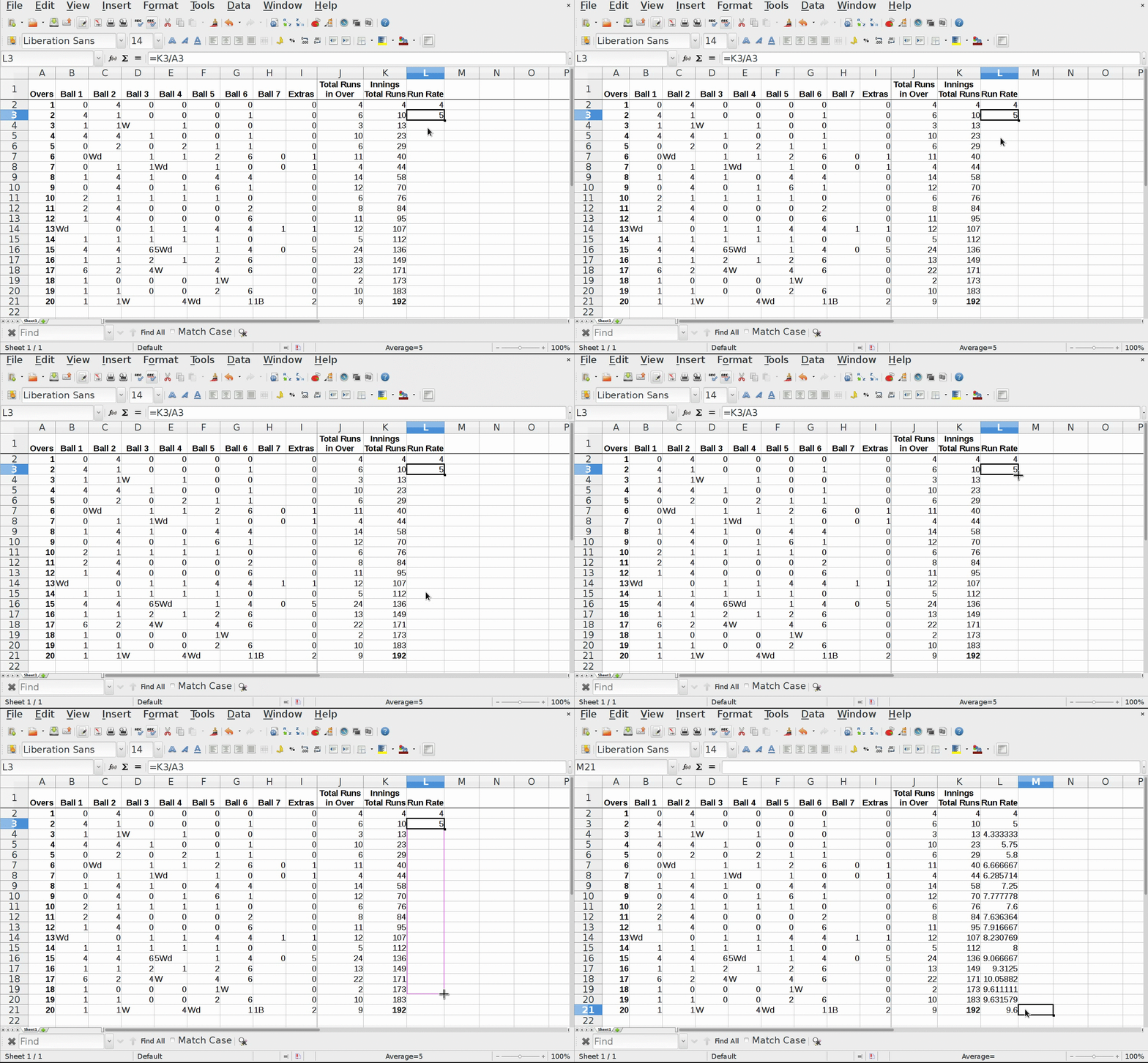
- Select cell L3 and enter the formula as =(K3/A3) and press "enter" button.
- Run rate after 2nd over will get reflected.

- Now drag the tiny rectangle of selected cell to reflect formula output for remaining overs.

Related Help Topic
Freezing Row/s
Go back to activity
×
Fixing column name row on scrolling of other rows (Freezing row):
- On mouse scrolling, column names row becomes invisible, since it goes upward.
- What if we want column names row to be visible even on scrolling as well.
- We can fix the column names row.
- Select the next row, after column names row using mouse's left click.
- Go to top most menu bar.
- Go to menu “Window -> Freeze” and click on it.
- This will freeze the column names row.
-
So "freeze function" fixes the rows, which are above the currently selected row.

Related Help Topic
Calculating total runs per over
Go back to activity
×
We can use inbuilt "SUM" function for summation.
Use cell range in "SUM(FirstCell:LastCell)" with the help of mouse selction:
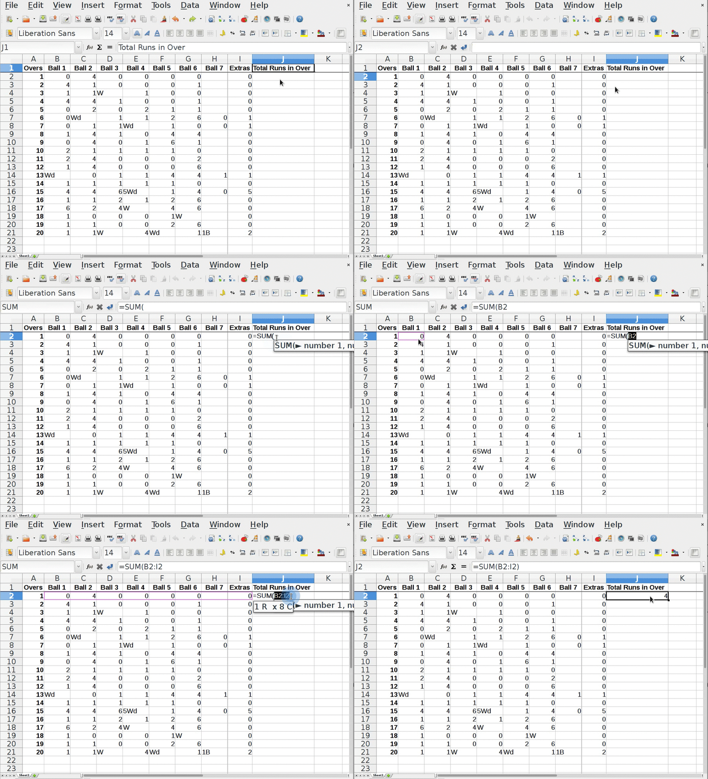
Use cell range in "SUM(FirstCell:LastCell)" with the help of mouse selction:
- Select cell J2, then enter the inbuilt function "SUM", by typing "=SUM("
- Then select the range of cells using mouse's pointer and left button, to drag and select those cells
- We can see the selected cell range gets reflected as =SUM(FirstCell:LastCell), Notice here "COLON" (:). For example: SUM(B2:I2)
- After cell range selection, press "Enter Key", and summation gets calulated.

Auto-completion for filling-up remaining overs total runs:
- Now use auto-completion feature to calculate remaining overs total
- Selecting cell "J2" and then drag tiny suare, till cell "J21"
- Total gets calculated by replicating same formula from cell "J2", by replacing corresponding row number.
Now we will make data entry and calculation, using the that tabular structure.
The scorecard for reference is given below.